Common Formulas
INDIRECT, ADDRESS, SORT, SORTBY, LET, SEQUENCE, INDEX, COLUMNS, ROWS, FILTER INDIRECT Calculations
Sometimes we would like to craft a formula acting on a range of cells where the specific cells we’d like the formula to act on are themselves determined by a formula. To deal with scenarios like this, INDIRECT is useful (for example, =INDIRECT("A1") returns the same thing as =A1).
Many guides caution against gratuitous uses of INDIRECT, and I am inclined to agree that whenever easy workarounds are available, they should be utilized. However, at least in versions of Excel more recent than 365, concerns about performance due to multiple calculations are overblown, at least from what I’ve seen. Without any issues, I have created sheets with thousands of separate INDIRECT functions working on an array with hundreds of thousands of datapoints.
A concrete example of where INDIRECT may come in handy is in performance calculations where new data is continually added to a data frame (the starting and ending row of “three years ago” changes as time goes by, after all). See the below example for reference. We have a data frame that is being continually updated and are trying to find the annualized return of the SPY ETF over different start dates. To do so, we tell Excel to get the geometric mean from the cell of the inception date to the cell of the last date in the range, and proceed to annualize the number (that’s the ^12-1at the end of the formula).
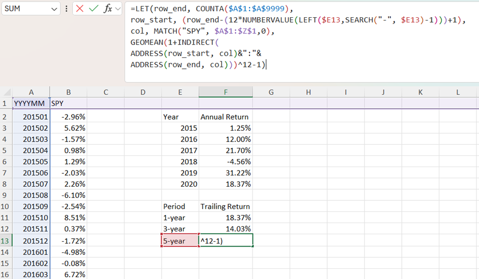
To make the formula more readable, we use LET. The last row in our data frame is just the count of all the rows in the frame (COUNTA($A$1:$A$9999)). The first row depends on the trailing return we want—since we are using monthly returns, the trailing three-year return will be 35 rows before the last row while the trailing five-year return will be 59 rows before the last row (this step is why we want to use INDIRECT in the first place). We can extract the number of rows we want to subtract using some of the techniques described in other sections.
In order to make the formula robust, we can use MATCH to identify the column we want to search in (we could also hard-code the column with “B”&row_start&”:”&”B”&row_end inside the INDIRECT). With the starting and ending rows in hand, along with the column we want our range to be in, we can use ADDRESS to make our INDIRECT usable. ADDRESS takes a row and column number, and returns the cell number. For example, =ADDRESS(1,2) returns $B$1 and =ADDRESS(3,4) returns $D$3. Additional arguments to the ADDRESS function determine which cells, if any, are frozen. By default, both the rows and columns are absolute rather than relative references.
Putting things together, we are using INDIRECT on column_start&row_start&”:”&column_end&row_end, and then computing the geometric mean before annualizing our results.
Reshaping, Rearranging, And Appending Dataframes
For the purposes of presenting data, “wide” format is often preferred. For the purposes of data analysis, “long” format is preferred. We can transform between the two by creatively implementing SEQUENCE inside of LET. As a concrete example, see the below data frame consisting of car type (in H2:H4) and color (in I1:L1), along with the demand for each of the combinations of type and color. We can put this in “long” format with the following techniques.
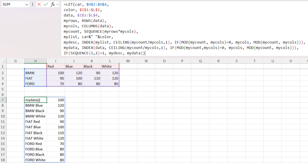
To make our code more readable and reduce repetition, we use LET. We store the demand for the type and color combo in a variable called data, the car type in a variable called car, and the car color in a variable called color. We use =ROWS() and =COLUMNS() to return the actual number of rows and columns of the data, and then (this is the step where we reshape the data frame) create a sequence of length equal to the number of data points.
Since “car” and “color” are dynamic ranges, we can combine them into a dynamic array (with “car” number of rows and “color” number of columns), which we call “mylist”. Our efforts now move to untangling the two arrays we have created. To do so, we INDEX them. The technique is replicated in both arrays, so we only discuss untangling the array which specifies the data.
In INDEXing, we want to change the row number only after we have exhausted all the columns. For example, with 12 data points and 4 columns, we only want to look in the second row after looking in the first row 4 times. A natural truck uses the CEILING function on division between the total number of data points (an array) and the number of columns (a fixed number). So, the first four values of the row array we use in INDEX are 1, the next four are two, etc.
#"data" is of size "myrows" by "mycols"#
#"mycount" is a sequence along the rows from 1 to length "myrows" times "mycols"#

= CEILING(mycount/mycols,1)                            #returns {{1}, {1}, {1}, {1}, {2}, {2}, etc.} down a column#
=INDEX(data, CEILING(mycount/mycols,1), ...)   #Returning the 1st row of "data" four times, then the second row four times, etc.#
A similar idea is used to change the column number. But with the rows now fixed, we want to iterate through the columns (so, 1,2,3,4 repeated 3 times, instead of 1 three times followed by 2 three times, etc.). To get this result, we use MOD instead of CEILING. In total, the first item we’re INDEXing is from the first row and first column of our dynamic array, the second item is from the first row and second column of the array, etc.
#"mycount" is a sequence along the rows from 1 to length "myrows" times "mycols"#
#here, mycount is of length 12, and mycols is 4#

=MOD(7,4)    =MOD(11,4)                                                              #both return 3, since 7=4*1+3 and 11=4*2+3#
=MOD(mycount, mycols)                                                                #returns {{1},{2},{3},{0}, {1}, {2} etc.} down a column#
=IF(MOD(mycount, mycols)=0, mycols, MOD(mycount, mycols))  #returns {{1},{2},{3},{4}, {1}, etc. } down a column#
=INDEX(data, CEILING(mycount/mycols,1), IF(MOD(mycount, mycols)=0, mycols, MOD(mycount, mycols)))
As a final step, we use SEQUENCE to arrange our result in the way we want (this time, a sequence along the columns rather than the rows). In the first column, we put our INDEXed results from the naming convention, and in the second column, we put the INDEXed results from the data.
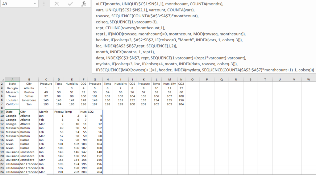
Another example of reshaping data is shown below:
Filtering Results
A powerful tool in newer versions of Excel is FILTER. One example where we might want to use this is shown below. The user has macro data on a process and has assigned ID’s to each item. The user would like each item to have data about both the category and sub-category of the item (and they know that, for example, if there are 10 items with category “A”, and 4 instances of sub-category “A1”, the 5th instance of category “A” will have sub-category “A2”).
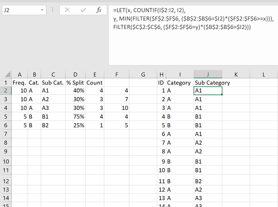
The usefulness of FILTER comes from combining conditions for FILTERing. Since arithmetic on TRUE/FALSE data automatically converts to numeric in Excel, we can use * (as a sort of “and”) and + (as a sort of “or”) to combine multiple filtering statements. In the above example, we first count the number of items that have categories that are the same as the current category up to the current selection (hence why we only freeze one row in COUNTIF(I$2:I2, I2)).
#Consider a range A1:A6 that has values A, B, A, B, B, A#
#Consider a value in B4 that is "B"#

=COUNTIF(A$1:A4, B4)   #returns 2#
We then examine the categories in the macro data that are the same as the current category and where the current sub-category’s incremental count are greater than our regular category count.
#Consider the same range A1:A6 that has values A,B,A,B,B,A#
#Consider further a range B1:B6 that has values 1,1,1,1,2,2#
#Finally, consider a value in C4 that is "B"#

=(A1:A6=C4)                                             #Returns {{FALSE}, {TRUE}, {FALSE}, {TRUE}, {TRUE}, {FALSE}}#
=(B1:B6>1)                                                #Returns {{FALSE}, {FALSE}, {FALSE}, {FALSE}, { TRUE}, {TRUE}}#
=(A1:A6=C4)+(B1:B6>1)                           #Returns {{0}, {1}, {0}, {1}, {1}, {1}}#
=(A1:A6=C4)*(B1:B6>1)                            #Returns {{0}, {0}, {0}, {0}, {1}, {0}}#
=FILTER(A1:A6, (A1:A6=C4)*(B1:B6>1))    #returns B#
Getting the minimum of this returned array, we can look at the macro data and select the rows which match both the category and incremental sub-category count. Note that we FILTER again on the category match, since different categories might have the same sub-category incremental sum.