Simulating Geometric Brownian Motion
We are considering the Geometric Brownian Motion \(d S_t = S_t(\mu \,dt + \sigma \, dW_t)\) where \(W_t\) is a Standard Brownian Motion and \(\mu\) (the drift term) and \(\sigma\) (the diffusion term) are fixed constants. We’d like to simulate this process using discrete approximations. We elect to use the first-order Euler-Maruyama Scheme (\(\widehat{S_{i+1}} = \widehat{S_i} + \mu \widehat{S_i} \Delta t + \sigma \widehat{S_i} \sqrt{\Delta t} Z_i\)) and the Milstein Scheme, a second-order refinement (\(\widehat{S_{i+1}} = \widehat{S_i} + \mu \widehat{S_i} \Delta t + \sigma \widehat{S_i} \sqrt{\Delta t} Z_i+\frac{\sigma^2}{2} \widehat{S_i} \Delta t(Z_i^2-1)\)). Here \(Z_i\) is an independent standard normal random variable and \(\Delta t = t_{i+1} – t_i = \frac{T}{N}\) where \(N\) is the number of observations and \(T\) is the time over which the Brownian Motion is observed.
(Exact) Probability Of Negative Values
Before embarking on our simulation, we’d like to ascertain certain properties of \(S_t\). In particular, we want to know \(\mathbb{P}(S_t < 0 | S_s > 0)\) for any fixed \(0 \leq s < t \leq T\); we want the probability the brownian motion goes negative in finite time given that it is positive at a certain point. By Ito’s Lemma, the analytic solution to the Geometric Brownian Motion is \(S_t=S_0 \exp{\left[\left(\mu-\frac{\sigma^2}{2}\right)t+\sigma(W_t-W_o)\right]}\) (and so \(S_t=S_s \exp{\left[\left(\mu-\frac{\sigma^2}{2}\right)(t-s)+\sigma(W_t-W_s)\right]}\)). Since the exponential term is always positive, and since we are conditioning on \(S_s > 0\), it is clear that \(\mathbb{P}(S_t < 0 | S_s > 0) = 0\) regardless of the specific values of \(s\) and \(t\).
(Simulated) Probability Of Negative Values
In contrast, there is a random variable in both the Euler-Maruyama (EM) and Milstein Schemes. For the simulations, we are interested in \(\mathbb{P}\left(S_{i+1}^N<0 \mid S_i^N >0\right) \) (here, \(N\) denotes the specific parameter combination of \(\mu\) and \(\sigma\) rather than an exponent). In the EM Scheme, this is exactly:
$$
\begin{align}
\mathbb{P}&\left( S_i^N+\mu S_i^N\Delta t+\sigma S_i^N \sqrt{\Delta t} Z_i <0 \mid S_i^N>0\right) && \text{Definition of EM Scheme}\\
&=\mathbb{P}\left(S_i^N\left(1+\mu \Delta t+\sigma \sqrt{\Delta t} Z_i\right)<0 \mid S_i^N>0\right) &&\text{Factoring}\\
&=\mathbb{P}\left(1+\mu \Delta t+\sigma \sqrt{\Delta t} Z<0 \right) &&\text{Conditioning, and $Z_i \stackrel{iid}{\sim}N(0,1)$}\\
&=\mathbb{P}\left(Z< -\frac{1+\mu\left(\Delta t\right)}{\sigma\sqrt{\Delta t}}\right) &&\text{Arithmetic}\\
&=\Phi\left(-\frac{1+\mu\left(\Delta t\right)}{\sigma\sqrt{\Delta t}}\right) &&\text{Where $\Phi$ is the standard normal CDF}
\end{align}
$$
While the added quadratic term makes the exact CDF a bit harder to come by in the Milstein Scheme, the same thought process as above shows that the probabilty the discretization is negative is non-zero. We have (noting \(Z^2>0\) and provided \(\sigma^2 \Delta t>(2\mu\Delta t+1) \)):
$$
\begin{align}
\mathbb{P}&\left(S_i^N\left(1+\mu \Delta t+\sigma \sqrt{\Delta t} Z_i +\frac{\sigma^2 \Delta t}{2}(Z_i^2-1)\right)<0 \mid S_i^N>0\right) &&\text{Definition of scheme}\\
&=\mathbb{P}\left(\left(\frac{\sigma^2 \Delta t}{2}\right)Z_i^2+\left(\sigma \sqrt{\Delta t}\right)Z_i+\left(1+\mu\Delta t-\frac{\sigma^2 \Delta t}{2}\right)<0\right) &&\text{Conditioning, and quadratic in $Z_i$}\\
&=\mathbb{P}\left(Z \in \left[\frac{-\left(\sigma \sqrt{\Delta t}\right) \pm \sqrt{\left(\sigma \sqrt{\Delta t}\right)^2-4\left(\frac{\sigma^2 \Delta t}{2}\right)\left(1+\mu \Delta t -\frac{\sigma^2 \Delta t}{2}\right)}}{2 \left(\frac{\sigma^2 \Delta t}{2}\right)}\right]\right) &&\text{Positive leading coefficient, so upward opening}\\
&=\mathbb{P}\left(Z \in \left[\frac{-\left(\sigma \sqrt{\Delta t}\right) \pm \sqrt{\sigma^2\Delta t\left(\sigma^2\Delta t-2 \mu \Delta t-1\right)}}{\sigma^2 \Delta t}\right]\right) &&\text{Simplifying discriminant}\\
&=\mathbb{P}\left(Z \in \left[\frac{-1 \pm \sqrt{\sigma^2\Delta t - 2 \mu \Delta t -1}}{\sigma \sqrt{\Delta t}}\right]\right) &&\text{Factoring $\sigma \sqrt{\Delta t}$}\\
&=\Phi\left(\frac{-1 + \sqrt{\sigma^2\Delta t - 2 \mu \Delta t -1}}{\sigma \sqrt{\Delta t}}\right)-\Phi\left(\frac{-1 - \sqrt{\sigma^2\Delta t - 2 \mu \Delta t -1}}{\sigma \sqrt{\Delta t}}\right) &&\text{Where $\Phi$ is the standard normal CDF}
\end{align}
$$
So, in both the EM Scheme and the Milstein Scheme, the probability of negative values does not depend on either \(S_i^N\) or the specific \(i\) (just the paramters \(\mu\) and \(\sigma\), and the step-size \(\Delta t=\frac{T}{N}\)).
Monthly Simulation Using EM Scheme
We’d now like to simulate the Brownian motion over the course of a year using monthly prices. We generate \(M=10^6\) paths of \(S_t\) using the Euler-Maruyama Scheme with \(N=12\) observations for each path, and repeat this procedure \(n=9\) times over, varying the parameter values \(\mu\in \left[-0.5, 0.5\right]\) and \(\sigma \in \left(0, 1.5\right]\) for each \(n\). Specifically, we use combinations of \(\mu \in \left\{-0.5, 0, 0.5\right\}\) and \(\sigma \in \left\{0.01, 1, 1.5\right\}\). A single sample path of the Brownian Motion is shown in Figure 1.1, and a small section of the \(M=10^6\)paths is shown in Figure 1.1.

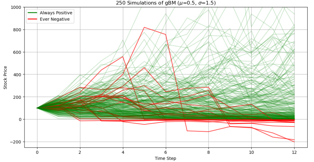
Modifications In EM Schemes To Avoid Negatives
To avoid negative values, there are a few immediate modifications to the above schemes that stand out. In cases where our estimated volatility is small (such as \(\sigma=0.01\)), this may not even be a concern, since the probability of going negative is miniscule. This is because the denominator in \(\Phi\left(-\frac{1+\mu\left(\Delta t\right)}{\sigma\sqrt{\Delta t}}\right)\) becomes small, and so the probability of getting a lower value than a large negative number with a standard normal is also small.
If such an estimate is not reasonable, than the easiest way to avoid negatives is to change the parameters of the simulation that we can directly control. For example, we can repeat the same simulation using daily data instead of monthly data. Checking the theoretical probability from the previous sections, \(\Phi\left(-\frac{1+\mu\left(\Delta t\right)}{\sigma\sqrt{\Delta t}}\right)\), we would anticipate the number of negative values to decrease since the square root term in the denominator grows smaller as \(N\) grows larger.
If this approach fails, we could always enforce a positivity condition by choosing a small positive number whenever the simulation goes negative. A more elegant option is to first transform our variable (move from geometric to arithmetic). We can then apply Itô’s Lemma to \(f(S_t)=\log(S_t)\) and see that \(d f(S_t)=(\mu-\frac{\sigma^2}{2})dt+\sigma dW_t\). Finally, we would use the same EM scheme to get a discretization, before transforming our values back with an exponential. This would ensure that our simulated values remain positive.
Code To Copy
###Load in required libraries###
import numpy as np
import pandas as pd
import matplotlib.pyplot as plt
import scipy as sp
###1a. Parameters For Monthly Prices###
t=1 #evaluate over interval [0,1] (can always re-scale)#
n=12 #the number of equally spaced time points (i.e. monthly data)#
dt=t/n #the increment of time#
M=10**6 #the number of times to redo the simulation#
N=len(mu)*len(sigma) #the number of times to run the simulation#
mu=np.array([-0.5, 0, 0.5]) #keep in [-0.5, 0.5]#
sigma=np.array([0.01, 1, 1.5]) #keep in (0, 1.5]#
s0=100 #initial stock price#
###1b. Generate A Bunch Of Randomness###
#use np.float32 to reduce storage demands#
#reusing the same normal matrix for different mu, sigma combos is fine#
np.random.seed(548)
z=np.random.normal(size=(n, M)).astype(np.float32)
###1c. Implement EM Scheme###
#reference specific simulation with biglist[list element][row, column]#
#e.g. biglist[2][:, 2] gives 3nd simulation of 3rd combo of mu and sigma#
biglist=[] #initialize#
for i in range(0,N): #Python starts at 0 instead of 1, and doesn't include last value in range (no comment...)#
a=i//len(mu) #the mu index, 0,0,0,1,1,1, etc. (// is floor division)#
b=i%len(sigma) #the sigma index: 0,1,2, 0,1, 2, etc. (% is mod)#
s=np.zeros((n+1, M), dtype=np.float32) #default is 64, want better storage#
s[0, :]=s0 #each simulation starts at s0#
geom_inc=(1+ mu[a]*dt + sigma[b]*np.sqrt(dt) * z) #since S_{i+1}=S_i*(geom_inc)#
s[1:, :] = s0 * np.cumprod(geom_inc, axis=0) #each i creates n+1 by M array#
biglist.append(s) #store each array in list#
print(biglist[2][:, 2].tolist()) #example simulation#
###1d. A single sample path#
combo=8 #the 9th parameter combo, mu=0.5 and sigma=1.5#
sim=10 #the 11th simulation (out of M) with this specific parameter combo#
s=biglist[combo][:, sim] #a single simulation#
plt.figure(figsize=(12,6))
plt.plot(s, color='blue', linewidth=1)
plt.title(f"Single Simulation of gBM ($\mu$={mu[combo // len(mu)]}, $\sigma$={sigma[combo % len(sigma)]})")
plt.xlabel("Time step")
plt.ylabel("Stock Price")
plt.grid(True)
plt.show()
###1e. A few sample paths####
from matplotlib.lines import Line2D #needed for legend (otherwise all paths get one)#
mysubsets=250 #the number of sample paths to examine#
combo=8
subset=biglist[combo][:, :mysubsets] #Look at first couple sample paths of mu=0.5, sigma=1#
plt.figure(figsize=(12, 6))
for i in range(subset.shape[1]): #shape[1] is number of columns#
col=subset[:, i]
if (col<0).any(): #Choose color of line based on if column contains negatives#
plt.plot(col, color="red", alpha=0.75) #alpha gives control over opacity#
else:
plt.plot(col, color="green", alpha=0.2)
mylegend = [
Line2D([0], [0], color="green", lw=2, label="Always Positive"),
Line2D([0], [0], color="red", lw=2, label="Ever Negative")
]
plt.title(f"{mysubsets} Simulations of gBM ($\mu$={mu[mycombo // len(mu)]}, $\sigma$={sigma[mycombo % len(sigma)]})")
plt.xlabel("Time Step")
plt.ylabel("Stock Price")
plt.ylim(-250, 1000)
plt.legend(handles=mylegend, loc="upper left")
plt.grid(True)
plt.show()
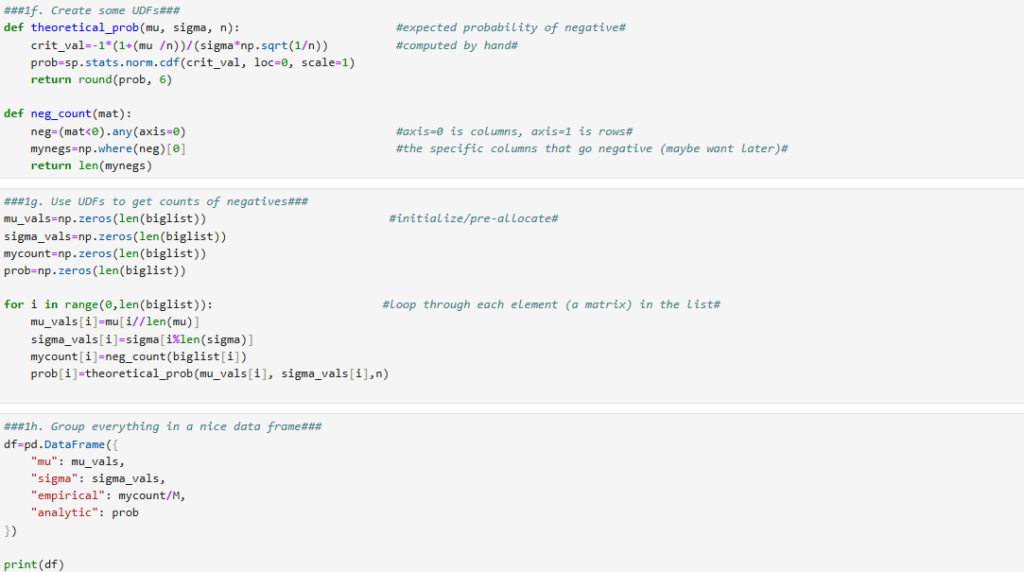
###1f. Create some UDFs###
def theoretical_prob(mu, sigma, n): #expected probability of negative#
crit_val=-1*(1+(mu /n))/(sigma*np.sqrt(1/n)) #computed by hand#
prob=sp.stats.norm.cdf(crit_val, loc=0, scale=1)
return round(prob, 6)
def neg_count(mat):
neg=(mat<0).any(axis=0) #axis=0 is columns, axis=1 is rows#
mynegs=np.where(neg)[0] #the specific columns that go negative (maybe want later)#
return len(mynegs)
###1g. Use UDFs to get counts of negatives###
mu_vals=np.zeros(len(biglist)) #initialize/pre-allocate#
sigma_vals=np.zeros(len(biglist))
mycount=np.zeros(len(biglist))
prob=np.zeros(len(biglist))
for i in range(0,len(biglist)): #loop through each element (a matrix) in the list#
mu_vals[i]=mu[i//len(mu)]
sigma_vals[i]=sigma[i%len(sigma)]
mycount[i]=neg_count(biglist[i])
prob[i]=theoretical_prob(mu_vals[i], sigma_vals[i],n)
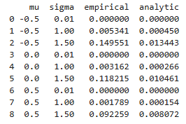
###1h. Group everything in a nice data frame###
df=pd.DataFrame({
"mu": mu_vals,
"sigma": sigma_vals,
"empirical": mycount/M,
"analytic": prob
})
print(df)