Common Formulas
IF, IFERROR, AND, OR, NOT, ISNUMBER, ISBLANK, AVERAGEIFS, SUMIFS, COUNTIFS, MAXIFS, MINIFSChaining IF Statements
One of the great things about Excel is that some of it’s most basic functions are also it’s most powerful. If-else statements (IF), error handling (IFERROR), conditional arithmetic (COUNTIF, AVERAGIFS, and SUMIFS), and other logic functions (AND, OR, and NOT) are all supremely useful.
Take the contrived example below. We input data in a trade log and want to record the realized profit for each trade. Of course, this information depends on a host of variables (are you buying or selling to open the trade? is it for an option contract or a stock?) so we’d like to address all the contingencies in one sweep.
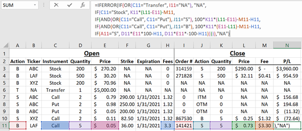
We do so by chaining together if statements, replacing the “else” logic with another IF statement. In the example, we first use the OR function to return “NA” when any statement inside the OR condition is met. On the second line, we get simple stock returns. On the third and fourth line, we use the AND function to address cases where an options contract (the condition on column C) is closed before expiration (the condition on column J). On the last line, we are left with options contracts that are held to expiration; if you sold to open, the individual trade is positive, if you bought to open, the individual trade is negative. Finally, we wrap the entire result with an IFFERROR to maintain good practice.
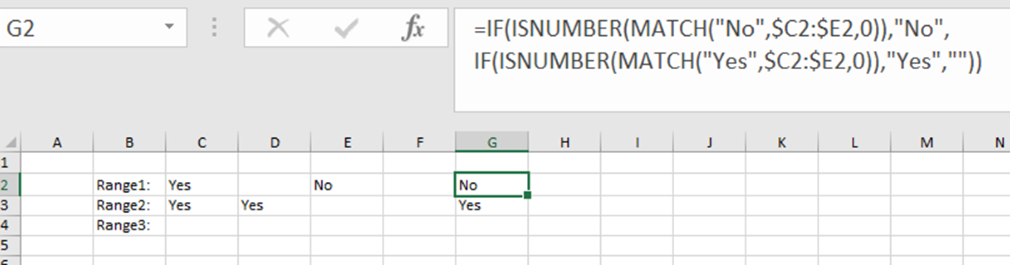
Utilizing ISNUMBER And ISBLANK
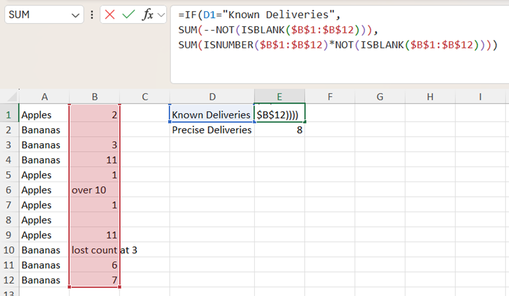
A nice trick that often comes up is using ISNUMBER and ISBLANK. As expected, the function returns TRUE if the argument is a number (blank), and FALSE otherwise. The below example demonstrates how these functions might be used.
We are given a range of data, some of which is blank, and some of which is non-numeric. Those cells which are left blank are assumed to be indeterminant—maybe there was a delivery, maybe there wasn’t. We can count the number of times we know that there was a delivery by inverting this count. We first generate an array of TRUE/FALSE data corresponding to whether or not the cell is blank (ISBLANK($B$1:$B$12)), then invert the TRUE/FALSE data with NOT(ISBLANK($B$1:$B$12)), then transforms the TRUE/FALSE to 1/0 data with --NOT(ISBLANK($B$1:$B$12)), before finally summing the resultant array. Since arithmetic on TRUE/FALSE data automatically converts the TRUE/FALSE to numeric, we can do a similar procedure to get the count of our data that has a precise number of deliveries (i.e. neither blank nor character data).
Some other implementations of these functions are shown below.
Conditional Arithmetic
Conditional arithmetic (e.g. sum this range, conditional on these conditions) is built into Excel with SUMIFS, AVERAGEIFS, and COUNTIFS. One thing to be aware of when using these functions is that conditioning on inequalities requires the use of quotations and the ampersand.
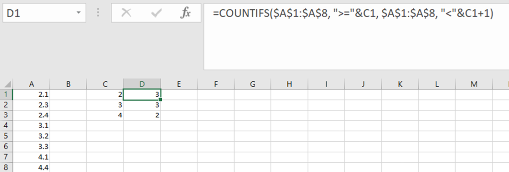
In the below example, we want to count the total number of observations that occur between integer values. One way to do this (another is the FLOOR and CEILING functions) is to use COUNTIFS (the extra S because we want to count based on more than one condition). In the cell below, we are counting the number observations that are at least 2 (note the quotation marks in $A$1:$A$8, “>=”&C1!) but strictly less than 3.
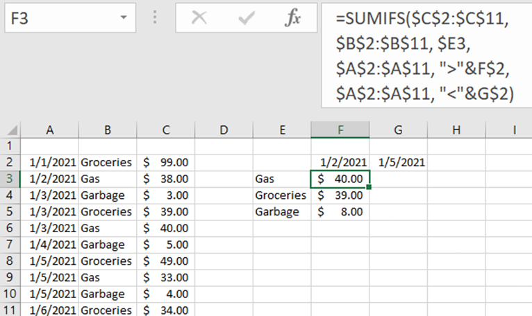
In general, the conditions do not need to be applied to the same range. For example, the below method to find the total amount of money spent on a given category over a given date range conditions uses three different ranges. We first condition on the category (we are only interested in the values that have value $E3in range $B$2:$B$11), then condition on the date (again using quotation marks and the ampersand, we are only interested in the values in range $A$2:$A$11 that are between F2 and G2), before finally summing the result over the column of money ($C$2:$C$11).
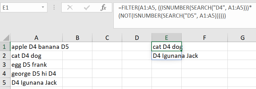
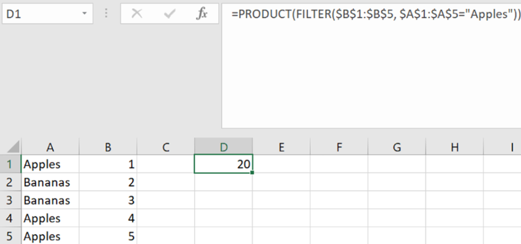
The advent of the FILTER function has made some of the conditional arithmetic redundant or outdated. For example, while there is no PRODUCTIF function, by combining PRODUCT and FILTER, we can make one that behaves similarly to what we’d expect. The below example filters the count portion of our data range ( $B$1:$B$5) based on name (we only care about the portion of the data that has “Apples” in the range ($A$1:$A$5), and then multiplies the result.
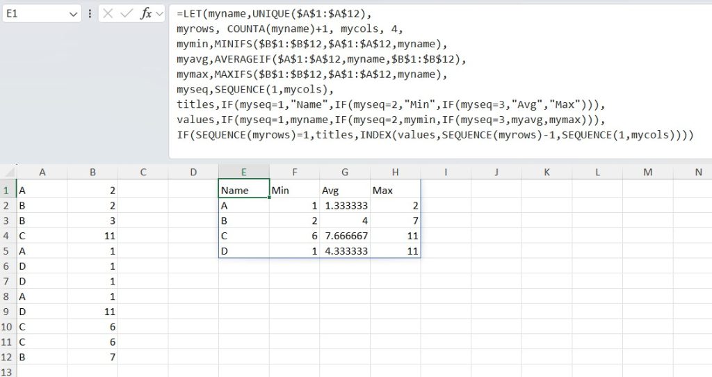
Finally, with a bit of help from LET (see the section on dynamic ranges), we can illustrate the behavior of some other conditional arithmetic, like MINIFS and MAXIFS.